Featured

5/recent

How to build Interactive Excel Dashboards

by June 02, 2018

How to build Interactive Excel Dashboards

How to build Interactive Excel Dashboards


How to build Interactive Excel Dashboards
In this video you will learn how to create an interactive dashboard from scratch using the built in Excel tools. No add-ins or VBA/Macros. Just plain Excel. Applies to Excel 2007 onward for Windows & Excel 2016 onward for Mac.

Download file used in the video
 with step by step instructions and links to more tutorials:

https://www.myonlinetraininghub.com/workbook-downloads


How to build Interactive Excel Dashboards


Download - How to build Interactive Excel Dashboards

Download

How to build Interactive Excel Dashboards:

How to Track Your Spending with Spreadsheet (2)

by October 04, 2017

Step by Step to Create Monthly Income & Expense Report

Here is the second part of Track Your Spending with Spreadsheet In Use. You can find the first part at How to Track Your Spending with Spreadsheet (1).

In this post, we will learn how to create the report check and track your income and expense in each month. The report will looks something like the capture below:

Google Sheet In Use: Monthly Income & Expense Report
Spreadsheet In Use: Monthly Income & Expense Report

The tracking recorded sample data Income & Expense Data look something like below image.

Income & Expense Data
Here, we will have one additional column to the first sheet in How to Track Your Spending with Spreadsheet (1), which is MONTH column. With this column, we will use the data from column A, Date, to generate month information. This will be talked about as below. This column play a very important role to enable you to view your income and expense monthly.

So we will have all together 8 columns as the detail below:
  1. The Date (Column A)
  2. Description (Column B)
  3. Type (income or expense) (Column C)
  4. The Amount (Column D)
  5. Actual Amount to track the sign of the amount (Column E)
  6. The balance (Column F)
  7. Optional Memo (just incase you would like to note something for reference later) (Column G)
  8. Month (Column H)

Generate Month Column

To generate the month information we will use the formula in H2 column:

=text(A2,"yyyy-mm")
or
=year(A2)&"-"&text(month(A2),"00")

This formula will generate the month in format yyyy-mm, where yyyy is 4 digits of year and mm is 2 digits of the month. The reason why year comes first in this format is when we do the report, the month and year will be in the correct order. You will see this when there are data more than one year.

Quick Formula Generating

One little trick to do a quick formula insert in every cell in H column from 2nd row to the last row of the information, follow these following steps:

  1. Copy (CTRL+C) H2 cell.
  2. Go to column F then press and hold CTRL key and at the same time press the down arrow key. This will take you to the last row. 
  3. Then, go to column H at that last row and hold down the SHIFT and CTRL key  and press up arrow key at the same time. This will select H column from last row to the first row. While still holding down the Shift and CTRL key click on H2 to select only the second row to the last row. 
  4. Paste the value (CTRL+V) you have copied from H2, you will have the data in H column ready there from the 2nd row to the last one. 

Note: CTRL key is COMMAND key in Mac OS

Now you are having your data ready to create monthly expense report.

Creating Monthly Income & Expense Report

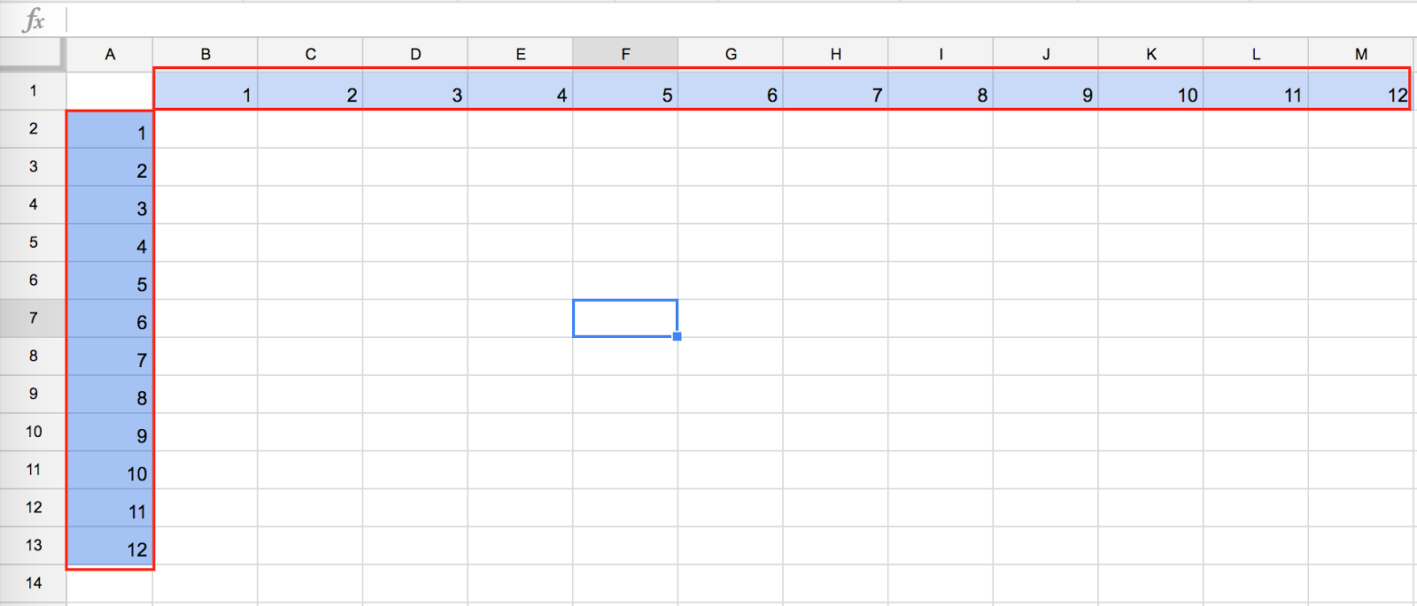
  1. Now go to A1 cell hold down  SHIFT and CTRL key and press right arrow key follows by down arrow key. With this step, you will select the whole information (data set).
  2. Go to menu Data and click at "Pivot Table" as the capture below.
    Spreadsheet in Use: Create Pivot Report 2
    Spreadsheet in Use: Create Pivot Report 
  3. Click at the report area to enable Report Editor at the right of the report.

    Spreadsheet in Use: Pivot Report Area
    Spreadsheet in Use: Pivot Report Area
  4. Select Description for RowsMonth for Columns and Actual Amount for Values with Summarize by as Sum. And you will have monthly Income & Expense Pivot report as below.
    Spreadsheet In Use: Monthly Income & Expense Pivot Report
    Spreadsheet In Use: Monthly Income & Expense Pivot Report
  5. To view the report differently, you can switch Rows and Column value and you will have the report as below.
    Spreadsheet In Use: Monthly Income & Expense Pivot Report 2
    Spreadsheet In Use: Monthly Income & Expense Pivot Report 2
Those are all necessary steps to create your month income & expense report with Spreadsheet in Use. To make the data more real, just adjust the number in each month for each item.

The data and example reports could be found at:


Please leave questions or feedback and please stay tune for my next tips and trick in Spreadsheet in Use. Thank you.

How to Track Your Spending with Spreadsheet (1)

by March 13, 2017

Spreadsheet in Use today, we brought you the trip on how to track your spending with spreadsheet. Have you ever come across the situation that at the end of the month you run out of your money and don't know what you have spent it on. Surprisingly, you will find yourself on the same boat with many others if your answer is a yes. If you want to get out of this boat, you should now start to track your spending. There was a saying that "When it comes to your purchases, what you don't know can hurt you". 

If you decide to track your spending then here is the trip to create a tool to do so with Spreadsheet with the very easy steps. 

Spreadsheet in Use: How to Track Your Spending with Spreadsheet

First thing you will need is the date that you spend your money, then the description of what has it been spent on. The amount that has been spent is also needed to be recorded. Apart from what you have spent your money on, you might as well would like to keep the track of your income a long with the expense. So I came up with 7 columns in the spreadsheet as follows:

  1. The Date (Column A)
  2. Description (Column B)
  3. Type (income or expense) (Column C)
  4. The Amount (Column D)
  5. Actual Amount to track the sign of the amount (Column E)
  6. The balance (Column F)
  7. Optional Memo (just incase you would like to note something for reference later) (Column G)

Next, In every of column E, you will need to keep a formula "=IF(C2="EXPENSE",-1,1)*D2".

Next, In cell F1, you will need to put a formula "=E2".

Next, In cell F2, you will need to put a formula "=F2+E3" and copy this cell to past to the the next one onwards (F3, F4, F5.....).

And as the picture can paint a thousand words, you can see them in the picture above or can take a look at the real spreadsheet example at Track Your Spending with Spreadsheet.

With this step, you will see what you have spent in each month. When you look back, you can see where and what your money went to and for. Even you can't fix it in the past, but you can plan for the future.

With this information we can view the information with pivot report as below:

Spreadsheet in Use: Spending Pivot Report
Spreadsheet in Use: Spending Pivot Report 1

To create this report, go to menu Data and click at "Pivot Table" as the capture below.

Spreadsheet in Use: Create Pivot Report
Spreadsheet in Use: Create Pivot Report 2

Then you would be brought to the next tab with the blank report as the capture below.

Spreadsheet in Use: Create Pivot Report
Spreadsheet in Use: Create Pivot Report 3


Choose Date and Description for Rows, Type for  for Columns, Actual Amount ($) for Values and Type in Filter and filter out Blank value

Spreadsheet in Use: Create Pivot Report
Spreadsheet in Use: Create Pivot Report 4

Spreadsheet in Use: Create Pivot Report
Spreadsheet in Use: Create Pivot Report 5

You can check the pivot report from google sheets at Track Your Spending Pivot Report


How to create a truly Interactive Timeline with Google Sheets

by September 12, 2016
How to create a truly Interactive Timeline with Google Sheets

In this video you will learn how to engaging content and interactive timelines for your teaching and VLE(Virtual Learning environment) or Blog? This video is made by Flipped Classroom Tutorials

Using Google Sheets and TimelineJS you can create stunning and truly interactive Timelines, using information, images, video, audio and so much more.

Here is the link to the TimelineJS : http://timeline.knightlab.com


Spread Sheet with Multiplication Table

by July 31, 2016
These are 4 steps to create multiplication table of 12 x 12 from google spread sheet. This is to get you familia with basic google spread sheet and the magic $ sign. You can play around with the $ by putting it in front of column and row. For example, $B$2, B$2 or $B2 and see what happens to the result.

Note:
The $ sign will lock the position of the cell, i.e A1, B1, C1.....

  • $B$2 will lock the whole cell, when you try to copy it to a new cell it will not change with column or row
  • B$2 will only lock the row of that cell position while the column will keep changing.
  • $B2 will only lock the column of that cell position while the row will keep changing.

Google Sheet Link: Spread Sheet In Use : Multiplication Table


1. Key in number 1 to 12 from A2 to M2 as the image below
Spread Sheet with Multiplication Table - Figure 1


2. Key in =$A2*B$1 in B2 as the image below


Spread Sheet with Multiplication Table - Figure 2

3. Click at the right bottom conner of B2 and drag it down to B13 as the images below. The result will be like in Figure 4
Spread Sheet with Multiplication Table - Figure 3

Spread Sheet with Multiplication Table - Figure 4


4. Select B2 to B13 by clicking at B2 and hold down the shift key and then click at B13. Then Click at the right bottom conner of B13 and drag it down to M13 as the image below. The result will be like figure 6

Spread Sheet with Multiplication Table - Figure 5
Spread Sheet with Multiplication Table - Figure 6


Get Yourself Ready with Google Sheet

by July 31, 2016
Get yourself ready and familia with Google Sheet with Google Spreadsheets for Beginners course

This is Google Spreadsheets for Beginners course by Natalia Lemoyne. In this course you will learn how to create a Google Spreadsheet. She will cover the basics of spreadsheets in Google. You will also learn some formatting tools to make your spreadsheets visually better as well as some tips such as automation to save time.


Powered by Blogger.